This repository contains the code for the R Shiny app MSstatsShiny, which utilizes MSstats, MSstatsTMT, and MSstatsPTM to analyze proteomics experiments.
This tutorial will walk through the steps on MSstatsShiny for performing differential abundance analysis for a dataset from Fragpipe. We use a case study of a DIA experiment that was analyzed using the FragPipe computational tool. The dataset originates from a clear cell renal cell carcinoma (ccRCC) study described in this paper. In the original study, researchers from the CPTAC profiled tumor (T) samples, together with normal adjacent tissue (NAT) samples from each cancer patient, indicating a paired design.
All datasets for this tutorial can be found at this link
Install MSstatsShiny using the instructions below:
-
Download R - https://cran.r-project.org/. Note R version must be >= 4.4
-
Note: if on windows you must also install R Tools - https://cran.r-project.org/bin/windows/Rtools/
-
Optionally you can also install RStudio Desktop - https://posit.co/downloads/
-
-
Run R or RStudio (if downloaded)
-
In the console run the installation code (see below) (https://bioconductor.org/packages/release/bioc/html/MSstatsShiny.html)
if (!require("BiocManager", quietly = TRUE))
    install.packages("BiocManager")
BiocManager::install("MSstatsShiny")
- If this does not work due to a release 3.21 issue, you can install release 3.20 with the following 2 commands:
BiocManager::install(version = '3.20', force = TRUE)
BiocManager::install('MSstatsShiny', version = '3.20', force = TRUE)
- If you get a bug related to lme4, you can install the latest version of lme4 with the following command:
install.packages("lme4", type = "source")
- You can also install from Github with the following command:
devtools::install_github("Vitek-Lab/MSstatsShiny", build_vignettes = TRUE)
- MSstatsShiny can now be started by running
MSstatsShiny::launch_MSstatsShiny()in the console
The online application is located at http://www.msstatsshiny.com/. The online version is constrained to processing only input files smaller than 100 MB; therefore, we recommend processing large datasets using a local installation.
library(MSstatsShiny)
MSstatsShiny::launch_MSstatsShiny()
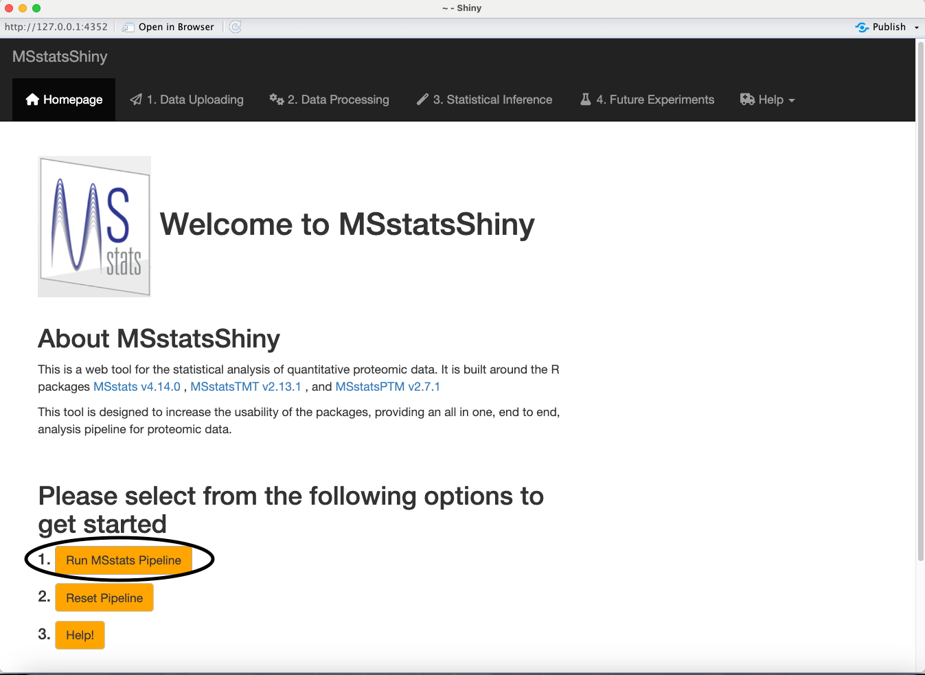
Click the Run MSstats Pipeline button to move to the data upload step.
-
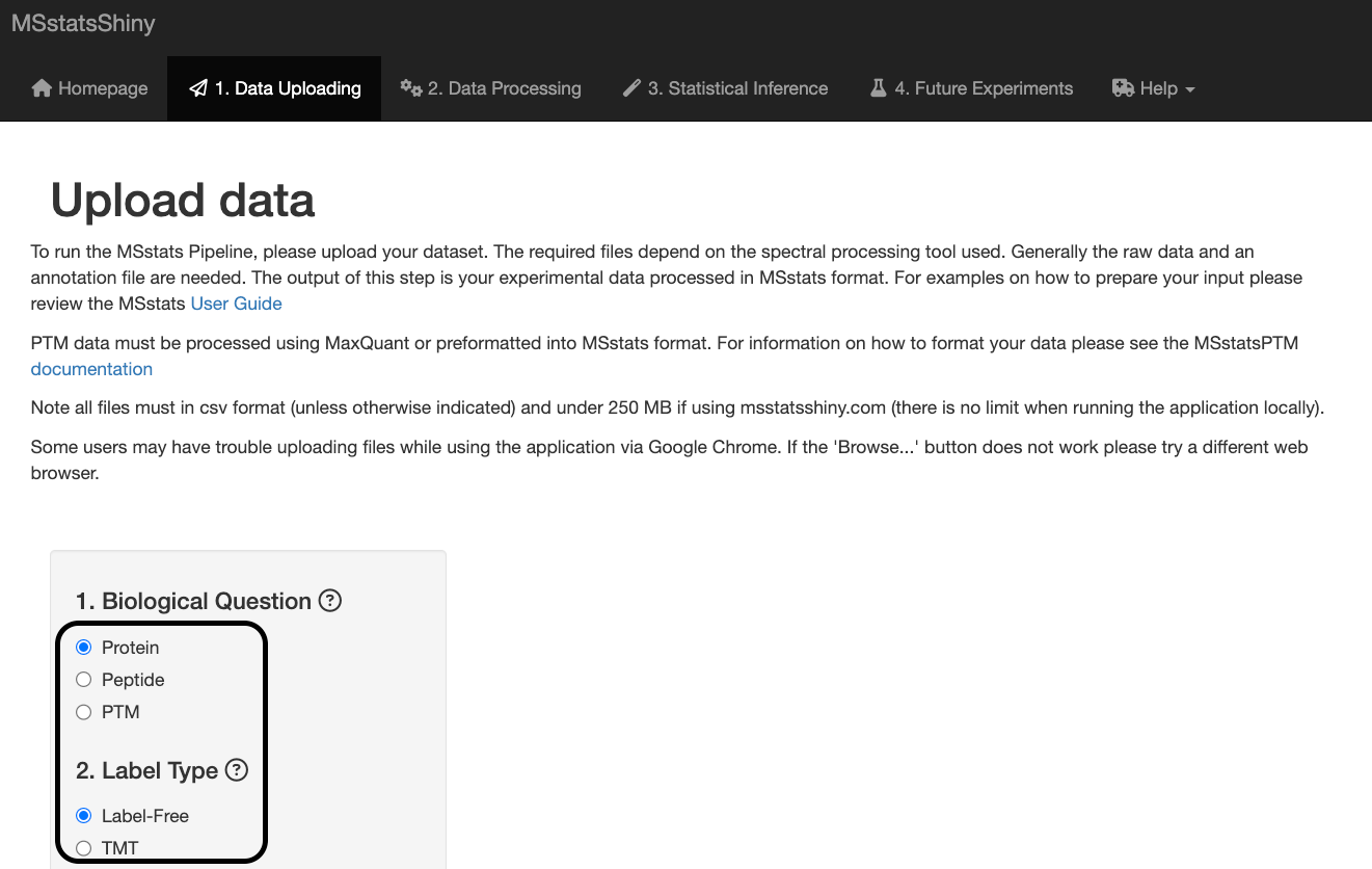
Biological Question:
-
Protein: Differential abundance analysis of proteins across conditions.
-
Peptide: Differential abundance analysis of specific peptides across conditions.
-
PTM: Differential abundance analysis of PTMs across conditions. See this paper for more information on how MSstatsPTM performs differential abundance analysis of PTMs via bottom-up MS proteomics.
-
-
Label Type:
-
Label-Free: Default setting associated with label-free DDA, DIA, SRM/MRM, PRM experiments
-
TMT: Use if your experiment uses tandem mass tags to perform sample multiplexing.
-
For this dataset, keep the default setting of Protein for the biological question and Label-Free for the label type.
This is where you select the tool that you used to produce ID/quant. For this case study, select Fragpipe for the type of file.
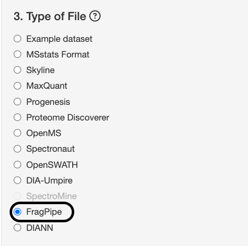
Each tool produces a quantification report that can be uploaded to MSstatsShiny to begin data conversion. For example, Fragpipe has this tutorial where you can export your quantifications in the format of MSstats.
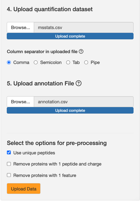
Upload msstats.csv from this link as the quantification dataset. Keep the default setting of comma for column separator.
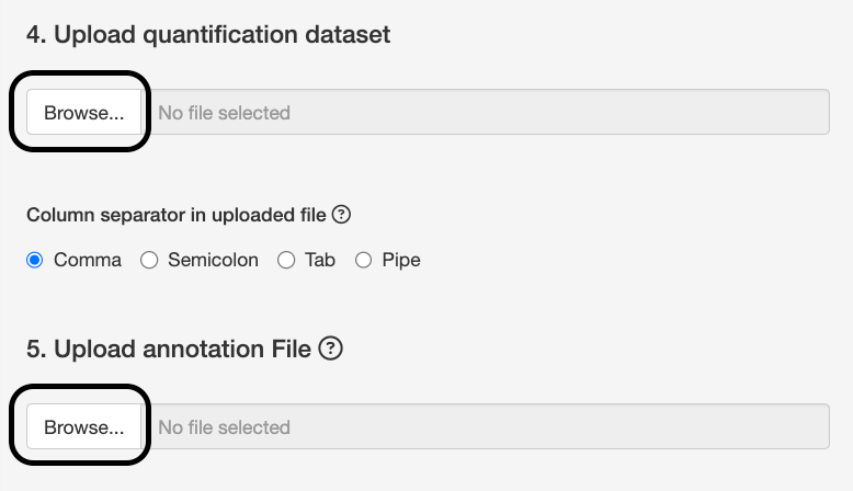
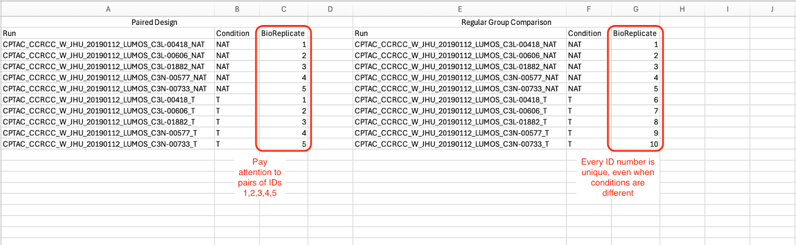
The annotation file defines the experimental design, notably which BioReplicate and Condition are associated with a particular MS run. You can see annotation.csv from this link as an example of an annotation file.
Because the experiment is paired, assign the same BioReplicate ID to the tumour and NAT runs originating from the same patient. This signals the paired design to MSstats. The image below illustrates how the annotation file is set up for paired designs.
-
Use unique peptides: If enabled, MSstats will remove any peptides that match with multiple proteins. Keep this option enabled.
-
Remove proteins with 1 peptide and charge: If enabled, MSstats will remove any proteins that have only 1 peptide quantified across all runs. We won’t enable this for now.
-
Remove proteins with 1 feature: If enabled, MSstats will remove any proteins that have only 1 peptide spectral match across all runs. We won’t enable this for now.
After attaching the dataset, the upload button should be enabled.
You should see a summary of your dataset and the top 6 rows of your dataset. Click Next step to proceed to data processing.
Because MS data is naturally left skewed, we log transform our intensities to bring intensities closer to a normal distribution. Although the distribution of our data may not be perfectly normally distributed after this transformation, the Central Limit Theorem guarantees that our statistical methods should perform adequately with any distribution given a large enough sample size.
-
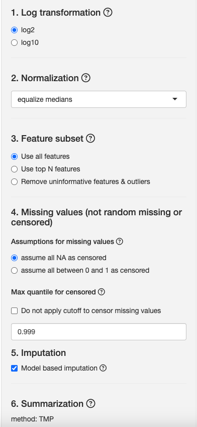
Log2: Transform intensities using a log2 scale. Keep this option selected.
-
Log10: Transform intensities using a log10 scale.
Reference: Kohler et al, Nature Protocols, 2024
-
Equalize Medians: Equalize medians of all log feature intensities in each run. NOTE: For SRM/PRM data, this option will normalize light-labeled peptides using heavy-labeled peptides as a global standard.
-
Assumptions:
-
All steps of data collection and acquisition were randomized
-
Most proteins in the experiment are the same and have the same concentration for all runs
-
The experimental artifacts affect every peptide in a run by the same constant amount
-
-
Effect:
-
The normalization estimates the artifact deviations in each run with a single quantity, reducing overfitting
-
The normalization reduces bias and variance of the estimated log fold change
-
-
-
Quantile: Equalize the distributions of all log feature intensities in each run
-
Assumptions:
-
All steps of data collection and acquisition were randomized
-
Most of the proteins in the experiment are the same and have the same concentration for all of the runs
-
The experimental artifacts affect every peptide non-linearly, as a function of its log intensity
-
-
Effect:
-
The normalization estimates the artifact deviations in each run with a complex non-linear function, potentially leading to overfitting
-
The normalization reduces bias and variance of the estimated log fold change but may over-correct
-
-
-
Global Standards: Equalize median log-intensities of spiked-in reference peptides or proteins. Apply adjustment to the remainder of log feature intensities.
-
Assumptions:
-
All steps of data collection and acquisition were randomized
-
The reference peptides or proteins are present in each run and have the same concentration for all of the runs
-
All experimental artifacts occur only after standards were added
-
The experimental artifacts affect every protein in a run by the same constant amount
-
-
Effect:
-
The normalization estimates the artifact deviations in each run with a single quantity, which reduces overfitting
-
The normalization estimates the artifact deviations from only a few reference peptides, which may increase over-fitting
-
The normalization does not eliminate artifacts that occurred before adding spiked references
-
The normalization reduces bias and variance of the estimated log fold change
-
-
-
None: Do not apply any normalization
-
Assumption:
-
All steps of data collection and acquisition were randomized
-
The experiment has no systematic artifacts or has been normalized in another custom manner
-
-
Effect:
- All patterns of variation of interest and of nuisance variation are preserved
-
For this case study, we will use the equalize medians option because we assume most proteins will not change in abundance across conditions.
Recall that a feature is a transition in SRM/PRM, a fragment in DIA, and a precursor in DDA for a particular peptide.
-
Use all features: Uses all features to leverage all available information to infer the underlying protein abundance.
-
Use top N features: Selects a pre-specified number of features with the highest average intensity across all runs for each protein.This option is useful if you believe that the features with lower average intensity are less reliable, or in cases where some proteins have an unusually large number of features (such as DIA experiments). For any individual protein, it is usually possible to determine changes in abundance by looking at the peaks with highest intensity; in these cases, using all features results in redundancy while greatly increasing the computational processing time.
-
Remove uninformative features & outliers: Attempts to select the ‘best’ features by removing features that have too many missing values, that are too noisy or have outliers.
For this case study, we will use all features, but later, we can use Remove uninformative features & outliers and assess profile plots & differences in differential abundance analysis results.
Different data processing tools have different ways of reporting missing values.
-
Assume all NA as censored: This option assumes that any NA value in the dataset is a value missing due to low abundance.
-
Assume all between 0 and 1 as censored: This option assumes that any log-transformed value between 0 and 1 is a value missing due to low abundance. NAs are treated as missing at random.
For our dataset, select Assume all NA as censored. Fragpipe only reports NAs, which we will assume are values missing at low abundance.
Reference: Figure 3 in Kohler et al, JPR, 2023.
-
Do not apply cutoff to censor missing values: If unchecked, all log intensities past a certain quantile will be marked as missing due to low abundance.
-
By default, this quantile is 0.1% quantile (defined using the value 0.999 in the image)
- To maximize the between-tools consistency of the analysis for low-abundant analytes MSstats learns, separately for each experiment and tool, a threshold for “high-confidence” log2-intensities. The threshold is a tuning parameter, defined as the 0.1th percentile of the log2-intensities in the linear regime of the dynamic range, and estimated as follows. Define qp the pth percentile of all the log2-intensities that exceed 0. In particular, the median is q50, the 25th percentile is q25, and the 75th percentile is q75 (dotted lines in Figure 3). MSstats estimates q0.1 as q0.1 = q25 - (q99.9 - q75)
-
For this study, we will leave this unchecked and keep the default threshold.
-
Model based Imputation [Checked]: Infer missing feature intensities by using an accelerated failure time model. It will not impute for runs in which all features are missing
-
Assumption: Features are missing for reasons of low abundance (e.g., features are missing not at random)
-
Effect: If the assumption is true, imputation will remove bias toward high intensities in the summarization step. Otherwise, bias will be introduced via inaccurate imputation
-
-
None: Do not apply imputation
-
Assumption: Assume no information about reasons for missingness or that features are missing at random
-
Effect: If the assumption is true, no new bias will be introduced. Otherwise, if features are missing for reasons of low abundance, summarized values will be biased toward high intensities
-
For this study, we will apply imputation. But we can also observe how intensities increase if we do not apply imputation.
- TMP: Tukey’s median polish is used to estimate protein level abundances from feature level abundances since it is robust to noise and outliers (in contrast to sum/mean normalization). This is the default setting.
- Remove runs with over 50% missing values: If enabled, this option removes the proteins where every run has at least 50% missing values for each peptide. We will keep this option disabled.
Click Run protein summarization to start processing your data. You should see a progress bar upon clicking.
After data processing is complete, click Update Summarized Results to see a table of summarized protein log intensity values.
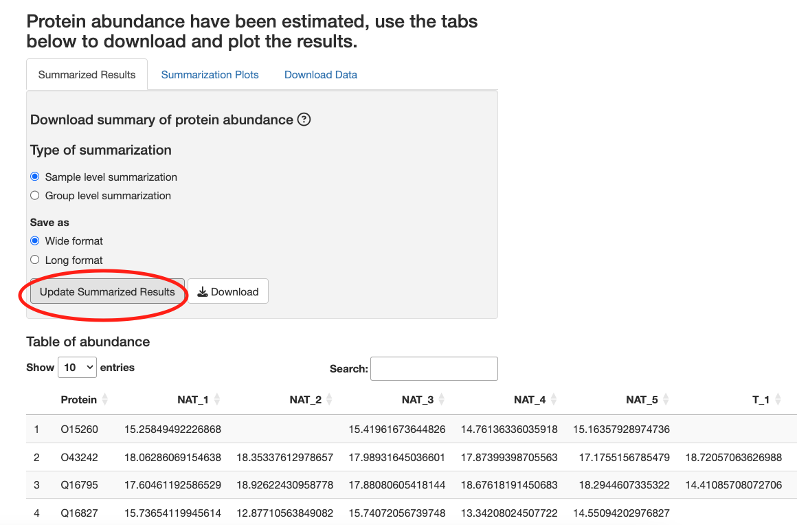
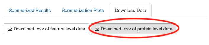
You can download protein and feature level intensity values at the Download Data tab.
On the Summarization Plots tab, there are two types of plots:
-
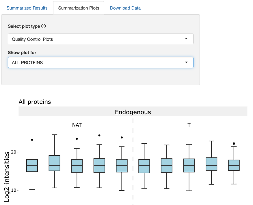
Quality Control Plots: This plot displays box plots of intensity values for each run. This plot helps with assessing the effects of normalization on a dataset.
-
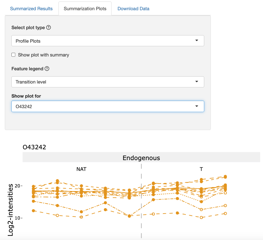
Profile Plots: This plot displays feature level intensity values for each run for a specific protein. This plot helps with assessing feature selection and missing values in a dataset.
We first assess QC plots. Under the Select plot type dropdown, click Quality Control Plots. Under the Show plot for dropdown, click the ALL PROTEINS option. We should expect to see the medians of these boxplots to be equal.
We next assess profile plots. Under the Select plot type dropdown, click Profile Plots.
Under the Feature legend dropdown, click the option Transition level. Under the Show plot for dropdown, click the protein O43242.
Lower-abundance features show greater variation and contain more imputed values, indicated by the open circles.
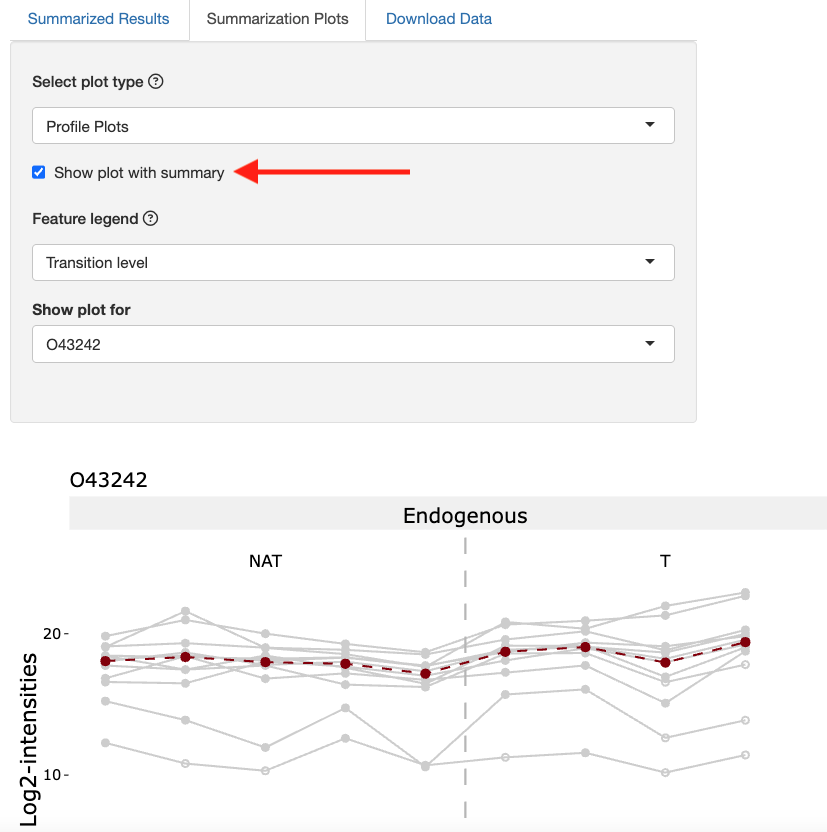
Click the checkbox show plot with summary. This will show the summarized value based on Tukey’s median polish for each run.
-
All possible pairwise comparisons: MSstats will perform differential abundance analysis on all pairs of conditions. For example, if you have 3 conditions A, B, & C, MSstats will perform analysis on A vs B, A vs C, and B vs C.
-
Compare all against one: User chooses one condition and MSstats performs differential abundance analysis on that one condition vs all remaining conditions. For example, if you have 3 conditions A, B, & C, and a user sets condition A to be compared against, MSstats will perform analysis on A vs B and A vs C.
-
Create custom pairwise comparisons: User chooses two conditions to compare against. For example, if you have 3 conditions A, B, & C, the user can choose to compare A vs B.
-
Create custom non-pairwise comparisons: User defines a contrast matrix. This is especially useful for more complex comparisons, e.g. comparisons with block designs.
For now, we will use Create custom pairwise comparisons to directly compare the control condition with the tumor condition. Click the Add button to confirm the contrast.
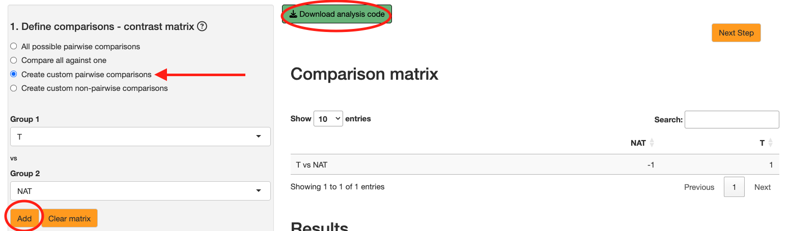
Note: You will also see a button at the top
Download analysis code. After performing statistical analysis, you can click this button to download the R code that was used to perform the whole analysis. This is useful for reproducibility and for users who want to run the analysis outside the Shiny app.
The significance level toggle acts as a filter to only proteins with an adjusted pvalue below a user-defined threshold. Next, click the Start button to begin the statistical analysis. This should trigger a progress bar.
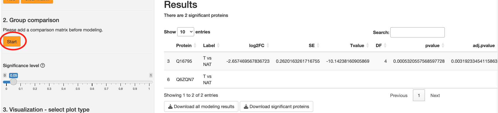
You should see a table to the right displaying the statistical results. There are the following columns:
-
Protein: The name of the protein for which the comparison is made.
-
Label: The label of the comparison, typically derived from the 'contrast.matrix'.
-
log2FC: The log2 fold change between the conditions being compared. The base of the logarithm is specified by the 'log_base' parameter.
-
SE: The standard error of the log2 fold change estimate.
-
Tvalue: The t-statistic value for the comparison.
-
DF: The degrees of freedom associated with the t-statistic.
-
Pvalue: The p-value for the statistical test of the comparison.
-
Adj.pvalue: The adjusted p-value using the Benjamini-Hochberg method for controlling the false discovery rate.
-
Issue: Any issues encountered during the comparison. NA indicates no issues. "oneConditionMissing" occurs when data for one of the conditions being compared is entirely missing for a particular protein, which can be particularly interesting to investigate further.
-
MissingPercentage: The percentage of missing features for a given protein across all runs. This column is included only if missing values were imputed.
-
ImputationPercentage: The percentage of features that were imputed for a given protein across all runs. This column is included only if missing values were imputed.
-
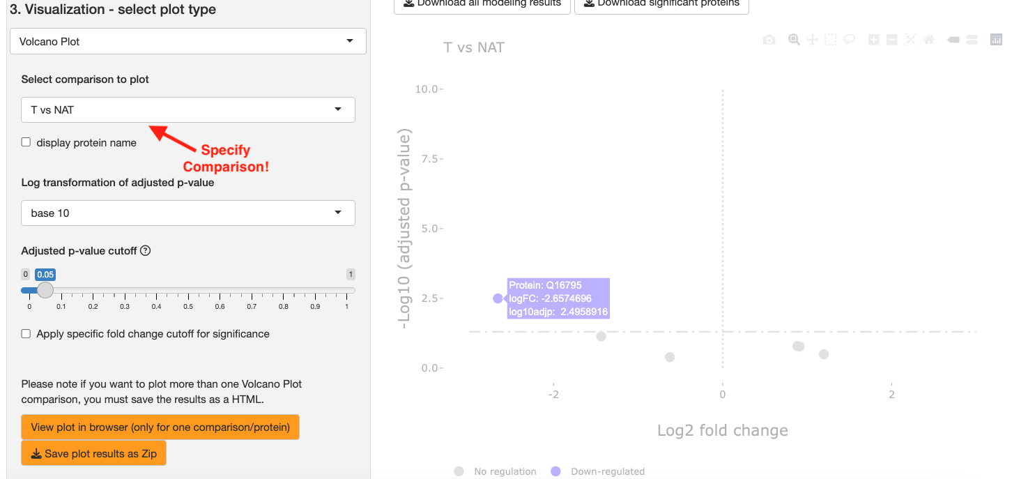
Volcano Plot: Generates an interactive volcano plot across all proteins for a specified comparison. Significant up-regulated proteins will be marked in red and significant down-regulated proteins will be marked in blue.
-
Heatmap: Generates a heatmap of logFCs across all proteins and comparisons. Useful for getting a high level view of which proteins to start investigating when there are multiple comparisons.
-
Comparison Plot: Plots a 95% confidence interval for a particular protein. Useful for verifying the uncertainty of a protein’s logFC and if its confidence interval crosses
For this tutorial, we will plot a volcano plot. Select Volcano plot as your plot type. Then select T vs NAT for the Select comparison to plot dropdown. Click View plot in browser to generate graphs.
Going back to the data processing step, take a look at the profile plots for protein Q16795.
Process the data again but with the Remove uninformative features & outliers option selected. Repeat steps 2-6 and observe what happens to protein Q5HYK3.
What do you notice about the differences in the profile plots? How does this affect the differential abundance analysis results?
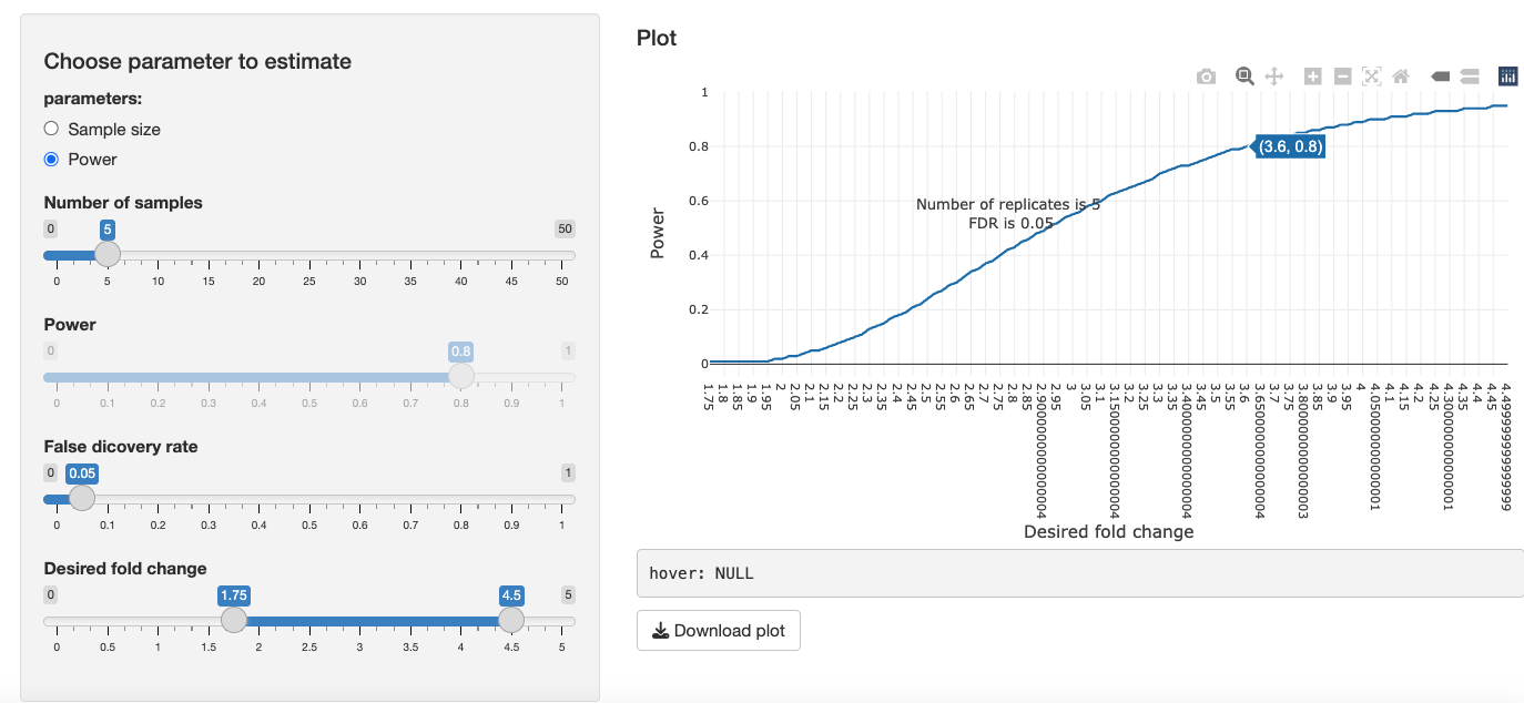
In the 4. Future Experiments tab, to illustrate the relationship of desired fold change and the calculated minimal number sample size to reproduce the desired fold change in a new experiment, we can consider 2 factors:
-
Power: The probability of detecting a significant protein when, in fact, the protein is significant.
-
FDR: The proportion of significant proteins that are false positives.
Tune the parameters of FDR and power. You will notice:
- As you increase power, sample size needed will increase.
- As you decrease FDR, sample size needed will increase.
- As your desired fold change decreases, the sample size needed will increase.
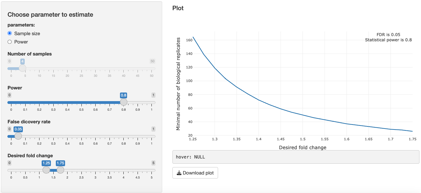
Switching to the power parameter, you can determine the power for a desired fold change given a predetermined sample size. This is especially useful if you're an experimentalist with a fixed number of samples and you want to know the power of your experiment to expect to detect a certain fold change.
To cite this application please use the corresponding publication in the journal of proteome research.
MSstatsShiny: A GUI for Versatile, Scalable, and Reproducible Statistical Analyses of Quantitative Proteomic Experiments
Devon Kohler, Maanasa Kaza, Cristina Pasi, Ting Huang, Mateusz Staniak, Dhaval Mohandas, Eduard Sabido, Meena Choi, and Olga Vitek. Journal of Proteome Research 2023 22 (2), 551-556 DOI: 10.1021/acs.jproteome.2c00603