mvgkde

MultiVariate Gaussian Kernel Density Estimator in JAX.

This is a micro-package, containing the single class MultiVarGaussianKDE (and helper function gaussian_kde) to estimate the probability density function of a multivariate dataset using a Gaussian kernel. This package modifies the jax.scipy.stats.gaussian_kde class (which is based on the scipy.stats.gaussian_kde class), but allows for full control over the covariance matrix of the kernel, even per-dimension bandwidths. See the Documentation below for more information.

Installation

pip install mvgkde

Documentation

For these examples we will use the following imports:

import jax.numpy as jnp
import jax.random as jr
import matplotlib.pyplot as plt
import numpy as np

from mvgkde import MultiVariateGaussianKDE, gaussian_kde  # This package

And we will generate a dataset to work with:

key = jr.key(0)
dataset = jr.normal(key, (2, 1000))

Lastly we will define a plotting function:

# Create a grid of points
(xmin, ymin) = dataset.min(axis=1)
(xmax, ymax) = dataset.max(axis=1)
X, Y = np.mgrid[xmin:xmax:100j, ymin:ymax:100j]
positions = np.vstack([X.ravel(), Y.ravel()])


def plot_kde(kde: MultiVariateGaussianKDE) -> plt.Figure:
    # Evaluate the KDE on the grid
    Z = np.reshape(kde(positions).T, X.shape)

    # Plot the results
    fig, ax = plt.subplots()
    ax.imshow(np.rot90(Z), cmap=plt.cm.gist_earth_r, extent=[xmin, xmax, ymin, ymax])
    ax.plot(dataset[0], dataset[1], "k.", markersize=2)
    ax.set(
        title="2D Kernel Density Estimation using JAX",
        xlabel="X-axis",
        xlim=[xmin, xmax],
        ylabel="Y-axis",
        ylim=[ymin, ymax],
    )

    return fig

Here's an example that can be done with jax.scipy.stats.gaussian_kde:

kde = gaussian_kde(dataset, bw_method="scott")

fig = plot_kde(kde)
plt.show()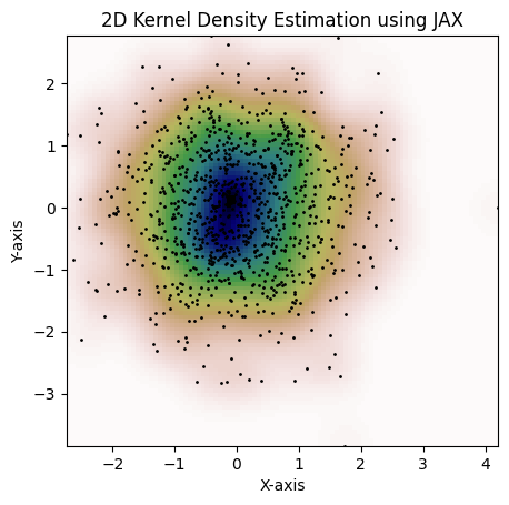

Here's an example with a per-dimension bandwidth. This is not possible with the jax.scipy.stats.gaussian_kde:

kde = gaussian_kde(dataset, bw_method=jnp.array([0.15, 1.3]))

fig = plot_kde(kde)
plt.show()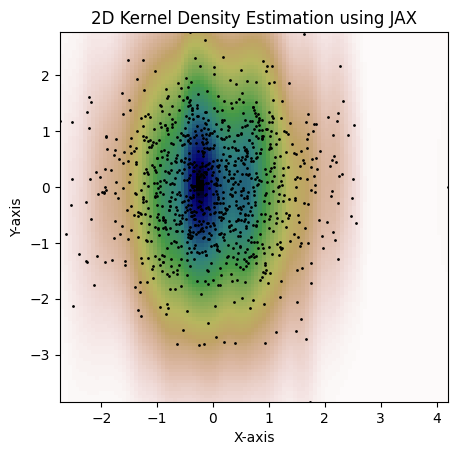

Lastly, here's an example with 2D bandwidth matrix:

bw = jnp.array([[0.15, 3], [3, 1.3]])
kde = gaussian_kde(dataset, bw_method=bw)

fig = plot_kde(kde)
plt.show()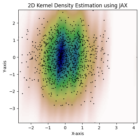

The previous examples are using the convenience function gaussian_kde. This actually just calls the constructor method MultiVariateGaussianKDE.from_bandwidth. This function allows for customixing the bandwidth factor on the data-driven covariance matrix, but does not allow for specifying the covariance matrix directly. To do that, you can call the MultiVariateGaussianKDE constructor directly, or the from_covariance constructor method. To illustrate the difference between modifying the bandwidth and setting the full covariance matrix, consider the following example:

kde = MultiVariateGaussianKDE.from_covariance(
    dataset,
    jnp.array([[0.15, 0.1], [0.1, 1.3]]),
)

fig = plot_kde(kde)
plt.show()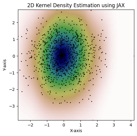

Acknowledgments

This package modifies code from JAX, which is licensed under the Apache License 2.0.